Building an NHL Playoff Pool Optimizer with Python
An end-to-end sports analytics project combining data engineering, statistical modelling, Monte Carlo simulation, and mixed-integer linear programming to optimize an NHL playoff pool roster.
This article focuses on the modelling decisions, methodology, and evaluation of the system I built and tested for the 2026 NHL Stanley Cup Playoffs. Links to the corresponding source code are provided throughout for readers interested in the implementation details.
Designing an Overly Complex Solution to Win a Family Competition
Introduction
Every year, my family runs an NHL Stanley Cup playoff pool. Participants draft a fixed roster of players before the playoffs begin, and earn points based on the performance of their chosen players throughout the postseason.
At first glance, choosing the best roster can seem simple enough: you pick the league’s best players from the best teams. In reality, team performance is inherently hard to predict and individual player point generation depends heavily on how long their teams survive in the playoffs. For example, a star player whose team is eliminated in the first round is worth less than a middle of the pack player who makes it to the finals. This makes roster selection an interesting problem involving prediction, uncertainty, and optimization.
This project is a system with the objective to:
- Simulate playoff bracket outcomes (Elo Rating & Monte Carlo Methods)
- Estimate each player’s expected playoff value (Statistical Modelling)
- Select an optimal fantasy roster (Linear Programming/Optimization)
- And most importantly, win the playoff pool (Bragging Rights).
While doing this might break the spirit of a fun family competition, it provides for an interesting project. I have also consistently done poorly in this playoff pool, so I clearly need to change my old strategy of hurriedly choosing players the day before the deadline.
The Optimization Problem
The rules of the playoff pool are quite simple. Before the start of the Stanley Cup Playoffs, each participant selects a roster which cannot be changed for the remainder of the tournament. The players on the roster obtain fantasy points, which are summed together and the highest fantasy score wins the pool.
Roster Constraints
- 15 skaters total
- 9 forwards
- 6 defencemen
- 2 goalies
Scoring
Skaters
- Goal: 2 Points
- Assist: 1 Point
Goalies
- Win: 1 Point
- Assist: 1 Point
- Shutout: 2 Points
Selecting a roster to maximize fantasy points requires answering three questions:
- Which teams are most likely to advance through the playoffs?
- Given those playoff outcomes, how many fantasy points is each player expected to score?
- Which combination of players maximizes the expected score while satisfying the roster constraints?
These questions naturally divide the project into major components which are discussed throughout this article.
System Overview
The system transforms raw NHL data (player statistics, team records, game results, etc.) into an optimized fantasy roster, given the above objectives and constraints. Each stage builds on the previous one, creating an end-to-end analytics pipeline. A high level overview of the system is represented in the following diagram.

Data Collection, Engineering, & Processing
The NHL provides two public APIs to access player statistics, game results, standings, schedules, and other information. While these APIs are well suited for individual queries, they appeared less convenient for large scale historical analysis, where thousands of requests must be made in a reproducible manner. I developed a small Python library to provide a clean interface for data collection. The library is responsible for:
- Constructing API endpoints
- Managing HTTP requests and sessions
- Automatic retries
- Caching raw API responses locally
- Returning structured JSON for downstream processing
This allows the analysis code to remain concise and modular to fit the needs of the project.
For example, retrieving the player statistics for an entire team’s roster requires only a few lines of code:
from nhl_pool.dataset.api import NHLAPI

api = NHLAPI()

params = {
    "abbrev": "MTL",
    "season": 20252026,
    "season_type": 2
}

data = api.get_team_roster_stats(params)
The library first checks if the requested data already exists in a local cache. If so, the cached response is returned immediately. Otherwise, the request is sent to the NHL API, the response is stored as a compressed JSON file, and the downloaded data is returned. The caching system was created to avoid unnecessary network requests, as it can be time consuming collecting a large number of records.
The processing of data was handled by scripts, which take the raw JSON files, flatten the nested API responses, and standardize them into tables such as:
- games.csv
- skaters.csv
- goalies.csv
- standings.csv
These processed datasets form the foundation for the remainder of the project.
For more detail on the implementation and processing pipeline, the source code is available on GitHub .
Predicting the Playoffs Outcome
The next challenge is estimating how the Stanley Cup Playoffs are likely to unfold. Since players can only accumulate fantasy points while their team remains in contention, predicting team performance is a critical component of estimating each player’s expected value.
To simulate the playoffs, we require a measure of team strength. While regular season standings provide an indication of performance, they are not suitable for predicting individual games. Instead, this project uses the Elo rating system, a method for estimating relative strengths of competing teams based on historical game results. These ratings can then be converted into win probabilities when comparing two teams, providing the foundation for simulating playoff brackets and estimating each team’s likelihood of advancing through the tournament.
Measuring Team Strength via Elo Rating
A notebook detailing the Elo implementation is available here .
The Elo Rating System
The Elo rating system is a method for calculating the skill or strength of a player/team relative to their competitors. The difference in ratings between two teams can be a predictor of the outcome of the game. A team with a higher rating is more likely to win against a lower rated opponent, while equally rated teams are expected to have an equal ability to win.
Algorithms
The base Elo system is defined by two algorithms.
The expected probability for team $A$, $E_A$, to win given the ratings of teams $R_A$ and $R_B$ is:
\[E_A = \frac{1}{1 + 10 ^ {\frac{R_B - R_A}{400}}},\]and similar for $E_B$. The factor of 400 is arbitrary and standard in Elo systems.
Given the actual outcome for team $A$, $S_A$:
\[S_A = \begin{cases} 1 & \text{if Player } A \text{ wins} \\ 0 & \text{if Player } A \text{ loses} \\ \end{cases},\]and
\[S_B = 1 - S_A,\]the rating of each team can be updated as:
\[R_A \gets R_A + K(S_A - E_A),\]and similarly for team $B$. The $K$ factor controls the sensitivity of the updates, with larger values producing larger rating changes after each game. A value of $K=20$ was chosen as a reasonable default, as it is consistent with values commonly used in Elo rating systems.
Extensions on the Elo System
The formulation above outlines the base Elo system, but a number of additions can be made to improve it.
Home Team Advantage
In sports there is said to be a benefit to the home team when they play at their home location.
Examining the results of all regular season NHL games between 2010-2025 showed that the home team won 54.10% of the time, demonstrating a slight advantage to the home team. We can try to account for this in the Elo ratings by giving the home team a slight rating boost, $h_{adv}$.
If we have two teams of equal strength, $R_A=R_B$, but the home team gets a boost of $h_{adv}$, then the expected win probability for the home team is (if $A$ is home team):
\[E_H = \frac{1}{1 + 10 ^ {\frac{R_B - (R_A+h_{adv})}{400}}} = \frac{1}{1 + 10 ^ {\frac{-h_{adv}}{400}}},\]Given the above analysis, $E_H = 0.5410$, and we can solve for $h_{adv}$, giving:
\[h_{adv} = -400\text{log}_{10}\left(\frac{1}{E_H} - 1 \right)\] \[h_{adv} \approx 30.\]This value is used when calculating Elo ratings in regular season games.
For playoff games over the same time frame the home team only won 51.31% of the time. This corresponds to $h_{adv} \approx 11$, and this factor is used when simulating playoff games.
Goal Differential
If a particular game was a blowout for example, we want the rating updates to reflect this as it could indicate one team is significantly stronger than the other. The World Football Elo Ratings have something called a “Goal Index”, $G$, where the number of goals between the winning and losing teams is taken into account. Football (soccer) scores are typically lower than hockey, so we’ll modify their update logic slightly.
For all regular season games in the dataset, I calculated the goal differential between the winning and losing teams and the results are visualized in the figure below.
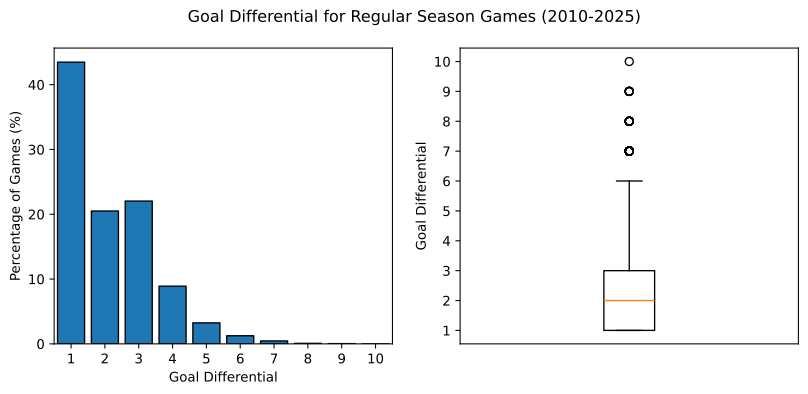
We see that approximately 65% of games have a 1-2 goal differential, and up to 85% of values are up to a goal differential of 3. Goal differentials greater than 6 are comparatively rare. Based on this empirical distribution, we can implement some logic for our goal index, $G$, as a function of the absolute goal differential, $N$.
\[G = \begin{cases} 1 & \text{if } N \leq 2 \\ 1.1 & \text{if } N =3 \\ 1.25 & \text{if } 4 \leq N \leq 5 \\ 1.5 & \text{if } N \geq 6 \\ \end{cases}\]Overtime and Shootout Wins/Losses
A game going to overtime or shootout are indicators that it was a close game, therefore the rating updates should be smaller in magnitude to reflect this.
We will use a simple factor of $M$ to implement this.
\[M = \begin{cases} 1 & \text{if game finishes in regular time} \\ 0.75 & \text{if game finishes in overtime} \\ 0.5 & \text{if game finishes in shootout} \\ \end{cases}\]Putting it All Together
Combining the modifications of the previous sections yields the final Elo formulation used throughout this project. Let $H$ denote the home team, and $A$ the away team.
The expected probabilities are:
\[E_H = \frac{1}{1 + 10 ^ {\frac{R_A - (R_H+h_{\text{adv}})}{400}}} \quad \text{and} \quad E_A = 1-E_H,\]The game outcomes are represented by:
\[S_H = \begin{cases} 1 & \text{if team } H \text{ wins} \\ 0 & \text{if team } H \text{ loses} \\ \end{cases} \quad \text{and} \quad S_A = 1 - S_H.\]The rating updates are:
\[R_H \gets R_H + KGM(S_H - E_H),\] \[R_A \gets R_A + KGM(S_A - E_A),\]where $h_{adv}$, $G$, and $M$ are the home-ice, goal differential, and overtime/shootout modifiers defined previously.
Calculating Elo Ratings
With the Elo system fully defined, we can now calculate Elo ratings using regular season box score data. At a high level, the Elo ratings are computed by repeatedly updating team ratings after each regular season game according to the following procedure:
- Initialize every team with an Elo rating of $R=1500$, the arbitrary but conventional initial value used in many Elo rating systems.
- Iterate through each regular season game in chronological order.
- Calculate the expected game outcome using the current Elo ratings.
- Update the Elo ratings based on the observed game result using the Elo update rules.
- Repeat steps 2-4 until every regular season game has been processed.
The final Elo ratings at the conclusion of the regular season are then used as the starting measure of team strength in the playoff simulations.
Results
The table below summarizes the ten highest rated teams according to the Elo system for the 2025-2026 regular season. For comparison, the final regular season league ranking is also shown.
| Team | Elo Rating | Elo Rank | Standings Rank |
|---|---|---|---|
| CAR | 1617.92 | 1 | 2 |
| BUF | 1613.01 | 2 | 4 |
| COL | 1603.33 | 3 | 1 |
| MTL | 1588.70 | 4 | 5 |
| OTT | 1576.24 | 5 | 9 |
| DAL | 1575.09 | 6 | 3 |
| TBL | 1572.35 | 7 | 5 |
| WSH | 1546.24 | 8 | 12 |
| MIN | 1544.06 | 9 | 7 |
| PHI | 1542.90 | 10 | 10 |
The ten highest rated teams finished the regular season with Elo ratings between approximately 1543 and 1618, indicating that the league’s strongest teams were relatively closely matched. Using the Elo win probability formula defined previously, a 75 point rating advantage corresponds to only an approximately 61% chance of winning a single game for the stronger team. This demonstrates the substantial uncertainty of game outcomes amongst even the strongest teams, motivating the use of Monte Carlo simulations rather than other strategies such as deterministic bracket prediction. For context, the lowest rated team at the end of the regular season was the Vancouver Canucks, with an Elo rating of approximately 1322.
The figure below shows the final Elo rankings and final regular season standings for all teams.
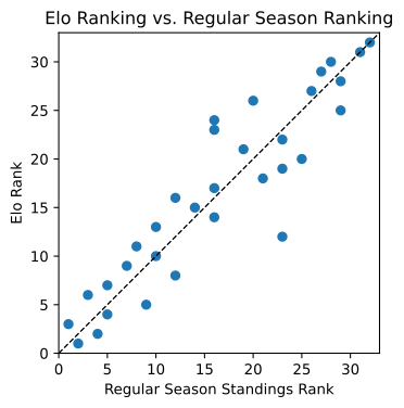
Overall, the Elo rankings broadly agree with the final regular season standings, with most teams lying close to the one-to-one line. This agreement provides confidence that the implemented Elo system produces reasonable estimates of team strength, while still distinguishing teams with similar regular season records.
The Elo ratings provide the foundation for estimating game win probabilities throughout the Stanley Cup playoffs, which will be further discussed in the next section.
Simulating Playoff Brackets with Monte Carlo Methods
A notebook detailing the playoff simulation framework is available here .
We can begin this section by acknowledging how difficult it is to accurately predict playoff bracket winners due to the uncertainty associated with each series. Even under the simple assumptions that every playoff series is a fair coin flip, there are
- Round 1: 8 series
- Round 2: 4 series
- Round 3: 2 series
- Stanley Cup Playoffs: 1 series
for a total 15 series, giving $2^{15}= 32,768$ possible playoff brackets without accounting for number of games played in each series.
Of course, playoff series are far from a coin flip-type result. Stronger teams are more likely to advance, and each possible bracket has a different probability of occurring based on the competing team strengths. Rather than attempting to predict a single “correct” bracket, this project instead simulates the playoffs thousands of times using the Elo derived win probabilities for each matchup.
Aggregating the results of these simulations provides estimates of each team’s probability of advancing through every playoff round, ultimately allowing us to estimate the expected number of playoff games played by every team.
Monte Carlo Methods
At a high level, a Monte Carlo simulation is a computational algorithm that uses repeated random sampling to obtain the likelihood of a range of results of occurring. They are a way to model the probability of different outcomes of a process that can not be easily predicted.
Simulating One Game
With the final Elo ratings calculated, simulating an individual game is straightforward. The home team’s win probability is first computed from the Elo ratings of the two teams. A uniformly distributed random number is then generated, and the game outcome is determined by comparing this value to the computed win probability. The implementation is shown below.
import numpy as np
rng = np.random.default_rng(seed=123)

def elo_compute_win_probability(R_h, R_a, h_adv=30):
    '''
    Given the Elo ratings, R,  for the home and away teams (h and a), compute the probability team h wins.
    h_adv: home team advantage factor.
    '''
    return 1.0 / (1.0 + 10**((R_a - (R_h + h_adv))/400.0))

def simulate_game(R_h, R_a, rng, h_adv=30):
    '''
    Returns a boolean 1 if home team won, otherwise home team lost.
    '''
    # Calculate the win probability of home team
    p_home_win = elo_compute_win_probability(R_h, R_a, h_adv=h_adv)

    # Random number
    u = rng.random()

    return u < p_home_win
Simulating the Entire Playoffs
With the ability to simulate an individual game, the next step is to simulate an entire Stanley Cup playoff bracket. Since each playoff matchup is a best of seven series, we first extend the game simulation to simulate an entire series using the standard 2-2-1-1-1 home ice format of the NHL. Games are simulated sequentially until one team reaches four wins, at which point the winner advances to the next round.
At a high level, one playoff simulation follows the procedure below:
- Simulate each first round series using the best of seven format.
- Advance the winning teams to the next round and determine the home team of the next series according to the NHL playoff format.
- Repeat for each round until the Stanley Cup Final has been simulated.
- Record the number of playoff games played by each team.
Repeating this process many times produces an approximation of the distribution of possible playoff outcomes. By aggregating the results across all simulations, we can estimate the expected number of playoff games each team will play.
Updating Elo During Simulation
Instead of holding the ratings static, for a playoff simulation we can update Elo ratings based on the simulated outcomes on each game in the simulation. This way we can try and capture team strength throughout the playoffs, for example a team going on a postseason hot streak can be represented with an increasing rating through the playoffs. At the beginning of each new playoff bracket simulation, the Elo ratings are reset to their values from the end of the regular season so that every simulated run remains independent of the others.
Results
A total of 200,000 Monte Carlo playoff simulations were performed. This was found to provide stable estimates for playoff outcome probabilities while remaining computationally inexpensive. We retain the results of each simulation and aggregate them once they are all complete. From this, the model produces our statistic of interest: the expected number of playoff games played per team.
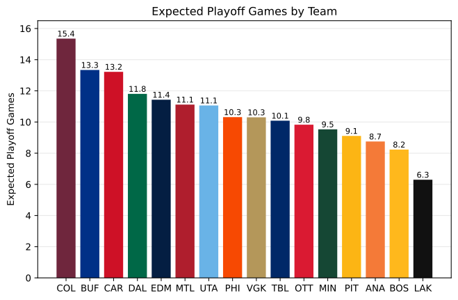
As a generality, the higher rated teams are projected to play more playoff games on average, reflecting their increased likelihood of advancing through multiple rounds of the postseason. Conversely, lower rated teams are expected to play fewer games due to their greater probability of early elimination. As a result of the starting playoff bracket being fixed, some strong teams are forced to play one another in the early rounds, while others benefit from a more favourable path through the bracket. These effects propagate throughout the tournament and influence the expected number of games played. The resulting expected game totals provide the link between the team level Monte Carlo simulations and the player level fantasy projections developed in the following section.
Although not as pertinent to the project, a fun byproduct of the simulations is that we obtain the probabilities of each team winning the Stanley Cup.
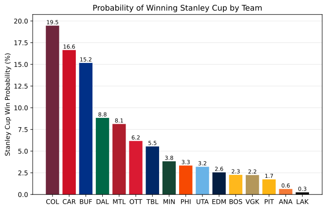
According to the simulations, the Colorado Avalanche emerge as the favourites to win the Stanley Cup with an estimated 19.5% chance of winning. Notably, no team exceeds a 20% probability of becoming champion, illustrating the uncertainty of the NHL playoffs, where even the strongest teams do not have a straightforward path to the Stanley Cup.
It is also interesting that the ordering of teams by Stanley Cup win probability differs from the ordering by expected number of playoff games. This reflects the fact that these two quantities measure different aspects of playoff success. For example, teams may be expected to play more games because they are projected to compete in longer series, while others may have a higher probability of winning the Stanley Cup despite playing fewer games on average. The fixed playoff bracket and resulting matchup structure contributes to these differences.
Estimating Player Value
Having estimated each team’s expected number of playoff games, we can now estimate the expected fantasy value of every player. This completes the predictive component of the pipeline and provides the inputs required for roster optimization.
For simplicity, we assume that each player will maintain their regular season scoring rate per game throughout the playoffs. While individual performance can certainly improve or decline in the postseason, regular season statistics provide a reasonable basis for expected production. Only statistics from the current regular season are used to estimate player performance. The per game expected value rates are then multiplied by the expected number of games played for the respective teams to obtain a player’s playoff expected value. We will more formally define this below.
Per the rules of the fantasy hockey pool, as explained in a previous section, skaters and goalies have different point systems.
Skaters
The scoring for skaters (forwards and defencemen) is defined as:
- Goals: 2 points
- Assists: 1 point
The expected playoff fantasy value, $\mathbb{E}[v_i]$, of skater $i$ is defined as
\[\mathbb{E}[v_i] = 2\,\mathbb{E}[G_i] + \mathbb{E}[A_i],\]where
\[\mathbb{E}[G_i] = \mathrm{GPG}_i \times \mathbb{E}[N_i],\] \[\mathbb{E}[A_i] = \mathrm{APG}_i \times \mathbb{E}[N_i].\]Here, $\mathbb{E}[G_i]$ and $\mathbb{E}[A_i]$ denote the expected number of goals and assists scored by skater $i$ in the playoffs, respectively. $\mathrm{GPG}_i$ and $\mathrm{APG}_i$ denote the skater $i$’s regular season goals and assists per game. $\mathbb{E}[N_i]$ denotes the expected number of playoff games played by skater $i$’s team.
Goalies
The scoring for goalies is defined as:
- Wins: 1 point
- Assists: 1 point
- Shutouts: 2 points
Similarly, the expected playoff fantasy value, $\mathbb{E}[v_i]$, of goalie $i$ is defined as
\[\mathbb{E}[v_i] = 2\,\mathbb{E}[\mathrm{SO}_i] + \mathbb{E}[W_i] + \mathbb{E}[A_i],\]where
\[\mathbb{E}[\mathrm{SO}_i] = \mathrm{SOPG}_i \times \mathbb{E}[N_i],\] \[\mathbb{E}[W_i] = \mathrm{WPG}_i \times \mathbb{E}[N_i],\] \[\mathbb{E}[A_i] = \mathrm{APG}_i \times \mathbb{E}[N_i].\]Here, $\mathbb{E}[\mathrm{SO}_i]$, $\mathbb{E}[W_i]$, and $\mathbb{E}[A_i]$ denote the expected number of shutouts, wins, and assists for goalie $i$ in the playoffs, respectively. $\mathrm{SOPG}_i$, $\mathrm{WPG}_i$, and $\mathrm{APG}_i$ denote the goalie $i$’s regular season shutouts, wins, and assists per game. $\mathbb{E}[N_i]$ denotes the expected number of playoff games played by goalie $i$’s team.
Assumptions
One complication of this methodology is that players can be traded throughout the regular season and may accumulate statistics for multiple teams. For the purposes of this project, a player’s regular season statistics are aggregated across all teams they played for, while their playoff expected values are determined using the team on whose playoff roster they ultimately appear. This assumes that a player’s scoring ability is independent of the team they played for during the regular season.
Optimizing the Roster
A notebook detailing the roster optimization implementation is available here .
Using the expected player values derived in the previous section, we can formulate the fantasy roster selection as an optimization problem. Before doing so, one practical consideration must be addressed. Since player value is estimated on a per game basis, players who appeared in a small number of regular season games could have inflated expected values due to small sample sizes. For example, a player who records three points and played in only one game would appear to have a fantastic scoring rate despite having little evidence that rate is sustainable.
To reduce the influence of these outliers, only players who appeared in at least 15 regular season games are considered by the optimizer. This threshold is empirical, but it removes many small sample anomalies while retaining players who regularly play.
Formulating the Mixed-Integer Linear Program
With the player pool defined, the roster selection problem can now be formulated as a mixed-integer linear program.
Participants select a fixed roster of players at the beginning of the playoff consisting of:
- 15 skaters total
- 9 forwards
- 6 defencemen
- 2 goalies
Decision Variables
For each player $i \in P$, where $P$ denotes the set of all players on playoff rosters, define the binary variable
\[x_i = \begin{cases} 1 & \text{if player } i \text{ is selected,} \\ 0 & \text{otherwise.} \end{cases}\]Objective Function
The objective is simply to maximize the total expected fantasy points accumulated by the roster.
\[\text{max}\sum_i \mathbb{E}[v_i]x_i.\]Here, $\mathbb{E}[v_i]$ is the expected fantasy value of player $i$, as defined in the Estimating Player Value section.
Constraints
The number of players in each position are our primary constraints, which can be written out as follows:
\[\sum_{i \in P} x_i = 17,\] \[\sum_{i \in F} x_i = 9,\] \[\sum_{i \in D} x_i = 6,\] \[\sum_{i \in G} x_i = 2,\] \[x_i \in \{0,1\}, \quad \forall i \in P,\]where $P$, $F$, $D$, and $G$ denote the respective sets of all players, forwards, defencemen, and goalies.
Additional strategic constraints can also be added into the optimization model.
A maximum number of players per team was imposed to encourage a more balanced roster and reduce the impact of incorrect playoff bracket predictions.
\[\sum_{i \in T} x_i \leq M_T \qquad \forall\ T,\]where $T$ represents the set of players belonging to a given team, and $M_T$ is the maximum number of players permitted from that team. A modelling choice of $M_T=8$ was implemented.
Furthermore, an additional constraint was imposed to prevent the optimizer from selecting more than one goalie from the same team.
\[\sum_{i \in G_T} x_i \leq 1 \qquad \forall\ T,\]where $G_T$ represents the set of goalies on team $T$.
Ideally, the goalie selected for the roster would be the starting goalie for that team.
Solving the Optimization Problem
The optimization model was implemented using SciPy’s scipy.optimize.milp solver. The expected player values define the objective function, while the roster requirements and strategic constraints are represented as linear equality and inequality constraints. Since milp is formulated as a minimization problem, the objective coefficients are simply negated to maximize the expected fantasy value.
The Final Roster
Finally, with all of the components of the project combined, running the linear programming optimizer yielded the following roster.
| Position | Player | Team | Expected Games | Fantasy Value/Game | Expected Points |
|---|---|---|---|---|---|
| FORWARD | |||||
| F | Nathan MacKinnon | COL | 15.35 | 2.25 | 34.54 |
| F | Martin Necas | COL | 15.35 | 1.77 | 27.16 |
| F | Connor McDavid | EDM | 11.43 | 2.27 | 25.93 |
| F | Leon Draisaitl | EDM | 11.43 | 2.03 | 23.21 |
| F | Nikita Kucherov | TBL | 10.08 | 2.29 | 23.09 |
| F | Jason Robertson | DAL | 11.80 | 1.72 | 20.30 |
| F | Tage Thompson | BUF | 13.34 | 1.49 | 19.92 |
| F | Cole Caufield | MTL | 11.11 | 1.72 | 19.08 |
| F | Wyatt Johnston | DAL | 11.80 | 1.60 | 18.86 |
| DEFENCE | |||||
| D | Cale Makar | COL | 15.35 | 1.32 | 20.26 |
| D | Evan Bouchard | EDM | 11.43 | 1.41 | 16.17 |
| D | Rasmus Dahlin | BUF | 13.34 | 1.21 | 16.11 |
| D | Shayne Gostisbehere | CAR | 13.22 | 1.15 | 15.14 |
| D | Darren Raddysh | TBL | 10.08 | 1.26 | 12.71 |
| D | Lane Hutson | MTL | 11.11 | 1.10 | 12.20 |
| GOALIE | |||||
| G | Scott Wedgewood | COL | 15.35 | 0.89 | 13.65 |
| G | Brandon Bussi | CAR | 13.22 | 0.92 | 12.20 |
| Total Expected | 330.52 |
Projected Team Total: 330.52 fantasy points
The roster composition by team is summarized below.
| Team | Players Selected |
|---|---|
| COL | 4 |
| EDM | 3 |
| DAL | 2 |
| BUF | 2 |
| MTL | 2 |
| TBL | 2 |
| CAR | 2 |
The optimized roster, as expected, primarily consists of players from teams projected to play the greatest number of playoff games. For example, the five teams with the highest expected games contribute 14 of the 17 selected players. At the same time, the optimizer does not simply select players from the tournament favourites. Instead, it balances expected playoff games with individual scoring ability. A notable example is Nikita Kucherov, who has the highest expected fantasy value per game and was selected despite Tampa Bay having the fewest expected playoff games amongst the teams selected.
Results
With the 2026 Stanley Cup Playoffs complete, we can compare the model’s projections against the actual fantasy points scored by the selected roster.
| Pos | Player | Team | Exp. Games | Actual Games | Exp. Points | Actual Points | Prediction Error |
|---|---|---|---|---|---|---|---|
| FORWARDS | |||||||
| F | Nathan MacKinnon | COL | 15.35 | 13 | 34.54 | 22 | -12.54 |
| F | Martin Necas | COL | 15.35 | 13 | 27.16 | 14 | -13.16 |
| F | Connor McDavid | EDM | 11.43 | 6 | 25.93 | 7 | -18.93 |
| F | Leon Draisaitl | EDM | 11.43 | 6 | 23.21 | 13 | -10.21 |
| F | Nikita Kucherov | TBL | 10.08 | 7 | 23.09 | 7 | -16.09 |
| F | Jason Robertson | DAL | 11.80 | 6 | 20.30 | 13 | -7.30 |
| F | Tage Thompson | BUF | 13.34 | 13 | 19.92 | 20 | +0.08 |
| F | Cole Caufield | MTL | 11.11 | 19 | 19.08 | 19 | -0.08 |
| F | Wyatt Johnston | DAL | 11.80 | 6 | 18.86 | 10 | -8.86 |
| DEFENCE | |||||||
| D | Cale Makar | COL | 15.35 | 13 | 20.26 | 9 | -11.26 |
| D | Evan Bouchard | EDM | 11.43 | 6 | 16.17 | 8 | -8.17 |
| D | Rasmus Dahlin | BUF | 13.34 | 13 | 16.11 | 18 | +1.89 |
| D | Shayne Gostisbehere | CAR | 13.22 | 19 | 15.14 | 15 | -0.14 |
| D | Darren Raddysh | TBL | 10.08 | 7 | 12.71 | 3 | -9.71 |
| D | Lane Hutson | MTL | 11.11 | 19 | 12.20 | 19 | +6.80 |
| GOALIES | |||||||
| G | Scott Wedgewood | COL | 15.35 | 13 | 13.65 | 7 | -6.65 |
| G | Brandon Bussi | CAR | 13.22 | 4* | 12.20 | 5 | -7.20 |
| Total | 330.52 | 209 | -121.52 |
* Brandon Bussi only played in 4 playoff games, while his team, the Carolina Hurricanes, played 19. Frederik Andersen turned out to be that team’s starting goalie for most of the playoffs.
A summary of the performance of the final roster is presented below.
| Metric | Value |
|---|---|
| Predicted Team Score | 330.52 |
| Actual Team Score | 209 |
| Prediction Error | 121.52 |
| Final Pool Rank | 13 / 38 |
The optimized roster was projected to score 330.52 fantasy points but ultimately scored 209 points, corresponding to an overestimation of approximately 122 fantasy points. This placed the roster 13th of 38 entries in the playoff pool. In the first and second rounds of the playoffs, my roster was consistently in the top five in the pool, largely due to the fact that the roster contained high scoring players from many teams. While 13th is a respectable result, it demonstrates that there is considerable room for improvement in the modelling approach. For reference, the winning team in the hockey pool had a total of 254 points.
One noteworthy observation is that replacing Brandon Bussi with Frederik Andersen (the two main goalies for Carolina) would have increased the roster total to 223 fantasy points, tying for 3rd place in the playoff pool. This is unfortunately a limitation since starting goaltenders are not explicitly identified. Bussi and Andersen played 36 and 35 games respectively in the regular season for Carolina, and it was not announced who would primarily be starting playoff games prior to the first game.
The figure below compares the simulated expected number of playoff games with the actual number of games played for each playoff team (left), together with the corresponding prediction errors (right).
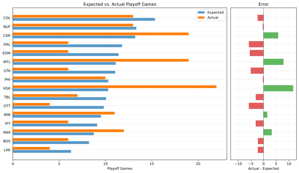
We see that the simulated expected number of playoff games tends to underestimate the teams that ultimately made deep playoff runs, most notably Vegas, Montreal, and Carolina in the figure above. This is reflected by the large positive errors shown in the right-hand panel. Conversely, many teams eliminated in earlier rounds have negative prediction errors, indicating that their playoff runs were overestimated. This is a consequence of the Monte Carlo simulation estimating the expected number of playoff games by averaging over many playoff brackets. As a result, the distribution of games played is compressed towards the middle. For example, Colorado was expected to play 15.4 games (the highest of any of the estimates) despite the fact that every Stanley Cup Finalist must necessarily play at least 16 games. Similarly, Los Angeles was the only team expected to play fewer than 7 games, even though 8 teams are guaranteed to be eliminated in the first round and therefore play at most 7 games. This averaging effect can systematically understate the fantasy value of players on teams that make deep playoff runs while overestimating the value of players whose teams exit early.
The figure below shows the fantasy point prediction error for every player selected in the optimized roster.
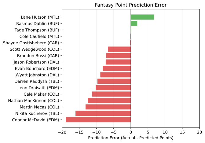
The prediction errors demonstrate how these team level playoff prediction errors propagated through the optimization model. Because expected player values were calculated using the simulated expected number of playoff games, the optimizer selected elite players from several teams that were all projected to make relatively moderate playoff runs. In reality, many of those projected runs did not materialize, leading to systematic overestimation across most of the roster. Conversely, players from Montreal, Carolina, and Buffalo generally met or exceeded their individual projections because their teams advanced as far as, or further than, expected. Although the players drafted from these three teams had lower expected value per game than many of the other players on the roster, their deeper runs ultimately resulted in higher total fantasy points. This finding could inform roster selection strategy: a solid player on a team making a deep playoff run (such as Lane Hutson) may be more valuable than selecting a superstar eliminated in the early rounds (such as Connor McDavid).
Overall, these results suggest that the dominant source of prediction error lies in forecasting team playoff advancement rather than modelling individual player performance. They also show a limitation of the current expected value formulation. By optimizing against the average outcome of many simulated playoff brackets, the model effectively selects players whose best outcomes occur in different, mutually exclusive playoff scenarios.
Future Work and Limitations
The results of this project highlights three areas that I think will most improve my chances in the next playoff pool:
- Strategy surrounding the optimization problem
- Improving the playoff simulation model
- Developing more accurate player value predictions
Optimization Strategy
My optimized roster this year contained players from seven different teams, providing strong production in the early rounds but causing large portions of the roster to be eliminated as the playoffs progressed. This was partially by design as I wanted to limit risk and hedge my bets and select a varied roster, hence the inclusion of the constraint of a maximum number of players allowed per team. Although the roster finished a decent 13th of 38 entries, only two players on the roster ultimately reached the Stanley Cup Finals.
For comparison, half of the pool’s winning team’s roster this year consisted of Carolina Hurricanes players (who went on to win the Stanley Cup). This suggests that the playoff pool rewards identifying a small number of teams that make deep postseason runs, even if that means selecting players with lower regular season production. This is a riskier and more aggressive strategy, but could be necessary to win the pool.
One possible modification to the optimization problem would be to limit the number of teams represented in the final roster (for example, two to four teams). If only two teams are selected, an additional constraint could require them to come from different conferences, ensuring both have a potential path to the Stanley Cup Final. Allowing up to four teams provides a balance between concentrating the roster on teams expected to make deep playoff runs and retaining some protection against incorrect playoff predictions. As demonstrated by this year’s results, playoff outcomes are inherently difficult to predict, so placing the entire roster on only two teams may introduce unnecessary risk if one or both are eliminated earlier than expected.
Further, since the Monte Carlo framework already generates a large number of simulated playoff bracket outcomes, these simulations could be used to evaluate alternative roster construction strategies. Rather than producing a single optimized roster, multiple potential rosters could be created under different optimization constraints (for example, changing the limit of teams to choose from). Each candidate roster could then be evaluated across the distribution of simulated playoff outcomes, allowing the strategy that performs best on average to be identified. This effectively introduces a layer of evaluation to the system, allowing the selection of a roster based on its expected value and on its robustness across many plausible playoff scenarios.
Improving Playoff Predictions
A more aggressive optimization strategy is only effective if the playoff simulations correctly identify the teams most likely to advance. While I believe the Monte Carlo simulation implementation itself is strong, several improvements to the underlying Elo model could potentially improve predictive performance.
- Optimizing the Elo parameters ($K$, $G$, and $M$) using a grid search or other hyperparameter tuning technique.
- Carrying Elo ratings across multiple seasons rather than reinitializing every team to 1500 at the start of a regular season, allowing long term strength of a team to persist.
- Introducing stochastic game-to-game performance variability during simulations to better capture inherent randomness in hockey.
Improving Player Value Predictions
The current implementation estimates playoff fantasy point ability directly from regular season statistics on a per game basis. This is a bit naive as it assumes that a player’s scoring rate remains unchanged in the playoffs, which is unlikely to hold in practice. I created some preliminary experiments with simple machine learning models which showed slight improvement in player value prediction over the current methodology, even with limited feature engineering. Additional development time could potentially improve this further.
However, I suspect improvements in player value modelling will produce smaller gains than improvements to the optimization formulation or playoff simulations. Once the optimization is constrained to a small number of teams, the selected players are likely to be the obvious high scoring players from those teams regardless of whether their expected values are estimated using a simple heuristic like this year or a more sophisticated machine learning model. Nevertheless, a stronger player value model would likely improve the overall robustness of the system so it remains an interesting objective for future work.
Closing Thoughts
So… after all that work, I still didn’t win.
While that is a bit of a bummer, I really enjoyed building this system from the ground up and putting my skills in software development, statistics, simulation, mathematical modelling, and optimization to the test (against the evidently superior hockey minds of my family). I look forward to trying again next year!
At the end of the day, this is just a fun family competition. I hope they do not mind too much that I am borderline cheating, even if I am still losing.